James N. McNair, Annis Water Resources Institute, Grand Valley State University

Lake metabolism is a set of coupled physiological processes carried out by the living component of lake ecosystems. It includes production of oxygen (O2) by splitting water molecules in the light reactions of oxygenic photosynthesis, uptake of carbon dioxide (CO2) and synthesis of simple carbohydrates in the dark reactions of oxygenic photosynthesis, synthesis of photoautotroph biomass from these simple carbohydrates and additional nutrients (e.g., nitrogen and phosphorus), consumption of dissolved organic matter and existing biomass by heterotrophic organisms to produce new biomass, respiratory uptake of O2 and production of CO2 by aerobic organisms, and several additional processes that usually are less important.

The mass of carbon taken up by oxygenic photoautotrophs in a lake over a specified period of time (e.g., one day or one year) is called gross primary production (GPP). The mass of carbon released by all aerobic organisms in a lake over the same period of time is called total respiration (R). The difference between GPP and R is called net production (NP = GPP - R) and tells us whether the living component of the lake ecosystem takes up more carbon as CO2 than it releases (so the lake is a net carbon sink) or less carbon than it releases (so the lake is a net carbon source) over the specified period of time. The lake is a net carbon sink if GPP > R (NP > 0) and a net carbon source if GPP < R (NP < 0).

Because of the very large number of lakes around the world (especially small lakes, which are the most productive), collectively they play a significant role in the global carbon cycle and in determining atmospheric concentrations of CO2, a major greenhouse gas (Cole et al., 2007; Tranvik et al., 2009). This fact underscores the importance of obtaining accurate estimates of GPP and R in lakes around the world. In collaboration with the Biddanda lab here at AWRI, we are working to improve these estimates through development of better models and statistical estimation techniques.

We are estimating GPP, R, and NP using the so-called free-water dissolved-oxygen (DO) method. This method requires (1) time series of measured DO concentrations and several other water-quality and weather variables, (2) a process-based model of DO dynamics in the lake, and (3) a statistical technique for estimating GPP, R, and NP using the measured time series and the model of DO dynamics.

We have developed a new statistical estimation technique that is more efficient than previous methods (McNair et al., 2013). Thus far, however, we have continued to use a standard and very simple type of model of DO dynamics in which it is assumed that the upper layer of water in a stratified lake is well mixed at all times and that there is no significant exchange between this layer and deeper water. Under these assumptions, it suffices to measure DO concentrations at a single depth (in this mixed layer) as the basis for estimating GPP, R, and NP. The overall procedure is diagrammed in Fig. 1.

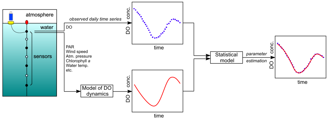
Figure 1. Schematic diagram of the overall modeling and estimation process.

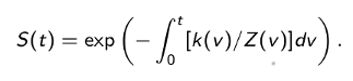
An example of a standard mixed-layer model of DO dynamics is shown below. We use separate equations for nighttime and daytime to avoid requiring light and dark respiration rates to be identical, since the underlying physiological mechanisms differ. The following symbols are used: C(t) is the DO concentration at time t, Ce(t) is the DO concentration in the mixed layer that would be in equilibrium with the atmosphere at the current water temperature and atmospheric pressure, r_N is the nighttime respiration rate, rD is the daytime respiration rate, k(t) is the gas transfer velocity for O2, Z(t) is the thickness of the mixed layer (called the mixing depth), p(t) is the flux of photosynthetically active radiation (PAR) within the mixed layer, and È is the the PAR-to-DO yield.

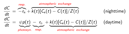
Once model parameters have been estimated used the measured time series (see below), GPP, R, and NP are computed using the following formulas:

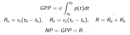
where nighttime begins at t0 and ends at tN, daytime begins at tN and ends at tD, RN and RD are nighttime and daytime total respiration, and GPP, R, and NP apply to one 24-h night-day cycle. These O2-based estimates are converted to carbon-based estimates using photosynthetic and respiratory quotients.

To estimate model parameters, the first step is to solve the differential equations governing nighttime and daytime DO concentrations. For the above model, we find:

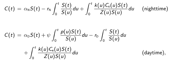
where

The next step is to discretize the integrals in the solution and consider the solution only at evenly-space times t0, t1, ... corresponding to the observed time series. Adding a statistical error term i to each discretized equation and putting Yi - C(ti), we obtain the following linear statistical models for nighttime and daytime DO concentrations:

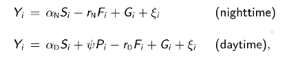
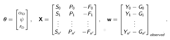
where Si, Fi, Gi, and Pi are discretized forms of the corresponding integrals in the above solutions. Using standard statistical theory for linear models, the least-squares estimates of model parameters are given in closed form by

where superscript T denotes matrix transposition and, for the daytime equation,

Because it is based on least-squares estimation, our approach does not requires us to assume a specific distributional form for the errors (residuals), nor does it require the errors to be serially uncorrelated. We also know that our least-squares estimators are unbiased. Another desirable feature of our approach is that we obtain exact, analytical expressions for our estimators, which permit us to compute numerical values directly and quickly rather than via iterative approximation.

The following are a few examples where we applied the above procedures to time series data for Muskegon Lake. We include examples where the mixed-layer model of DO dynamics accounts for observed dynamics very well and where it accounts for them poorly. We find that days where the model of DO dynamics accounts for observed dynamics poorly are very common in Muskegon Lake. Since the derived estimates of GPP, R, and NP cannot be trusted in such cases, it is important to determine why the model fails and to correct the problem(s). That is the focus of our current research.

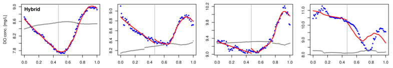
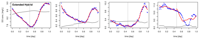
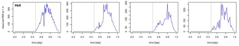
Figure 2. Examples of fitting four versions of the model of DO dynamics (rows 13) to Muskegon Lake time-series data for four different days (columns 14). Row 4 shows the PAR times series for reference.

Cole J. J., Prairie, Y. T., Caraco, N. F., McDowell, W. H., Tranvik, L. J., Striegl, R. G., Duarte, C. M., Kortelainen, P., Downing, J. A., Middelburg, J. J. & Melack, J. 2007. Plumbing the global carbon cycle: integrating inland waters into the terrestrial carbon budget. Ecosystems 10: 171–184.

McNair, J. N., Gereaux, L. C., Weinke, A. D., Sesselmann, M. R., Kendall, S. T. & Biddanda, B. A., 2013: New methods for estimating components of lake metabolism based on free-water dissolved-oxygen dynamics. Ecological Modelling 263: 251–263.

Tranvik, L. J. & 30 others, 2009: Lakes and reservoirs as regulators of carbon cycling and climate. Limnology and Oceanography 54: 2298–2314.

This work was partially supported by a grant from U.S. EPA Great Lakes Restoration Initiative.